Diagnostics
Overview
After fitting, the $sdtab data frame contains everything needed for standard goodness-of-fit diagnostics.
fit <- ferx_fit(ex$model, ex$data, method = "foce", covariance = TRUE,
                verbose = FALSE)
Mu-referencing detected for: ETA_CL, ETA_KA, ETA_Vsdtab <- fit$sdtabWe use method = "foce" here (matching the model file) because on this small dataset the FOCEI Hessian is not positive-definite and the covariance step fails. With FOCE the covariance step is computed and ferx_cor_matrix() returns a valid matrix.
The sdtab columns
names(sdtab) [1] "ID" "TIME" "DV" "PRED" "IPRED" "CWRES" "IWRES"
[8] "EBE_OFV" "N_OBS" "TAFD" "TAD" names(fit$ebe_etas)[1] "ID" "ETA_CL" "ETA_V" "ETA_KA"sdtab contains per-observation diagnostics. Per-subject ETAs are in fit$ebe_etas (one row per subject).
| Column | Location | Description |
|---|---|---|
PRED |
sdtab |
Population prediction (eta = 0) |
IPRED |
sdtab |
Individual prediction (fitted ETAs) |
CWRES |
sdtab |
Conditional weighted residual |
IWRES |
sdtab |
Individual weighted residual |
CMT |
sdtab |
Observation compartment — present only in multi-endpoint models (when any row has CMT != 1). Use this column to split GOF plots by endpoint. |
OCC |
sdtab |
Occasion index — present only in IOV models. |
CENS |
sdtab |
Below-LLOQ flag (0/1) — present only when the dataset has a CENS column. |
ETA_* |
fit$ebe_etas |
Empirical Bayes estimate (EBE) for each BSV parameter |
Core GOF plots
IPRED vs DV
ggplot(sdtab, aes(x = IPRED, y = DV)) +
  geom_point(alpha = 0.5) +
  geom_abline(slope = 1, intercept = 0, colour = "#1F6B7A", linewidth = 1) +
  labs(x = "IPRED", y = "Observed DV") +
  theme_minimal()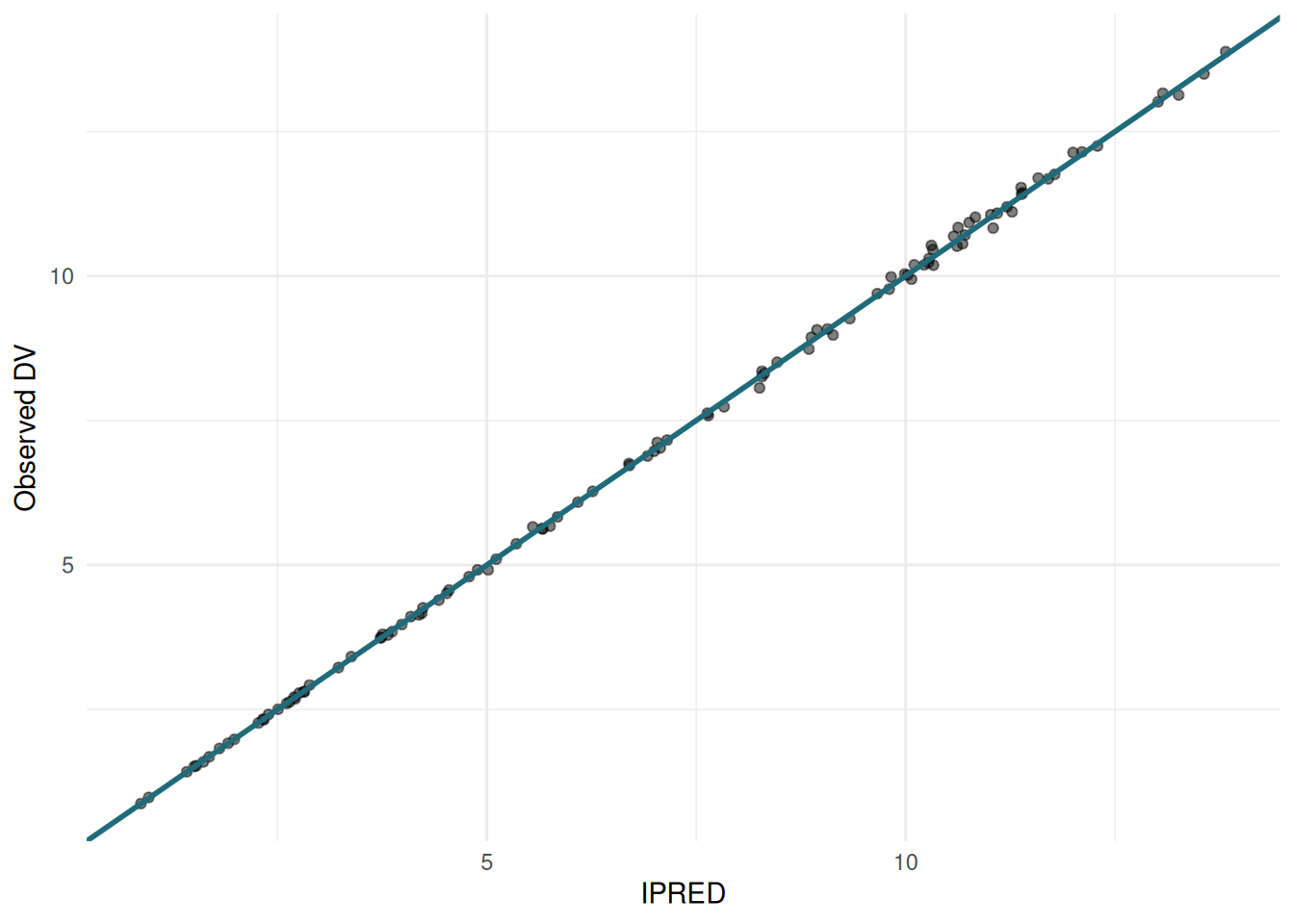
CWRES vs PRED
ggplot(sdtab, aes(x = PRED, y = CWRES)) +
  geom_point(alpha = 0.5) +
  geom_hline(yintercept = 0,      colour = "#1F6B7A", linewidth = 1) +
  geom_hline(yintercept = c(-2, 2), linetype = "dashed", colour = "#C8893E") +
  labs(x = "PRED", y = "CWRES") +
  theme_minimal()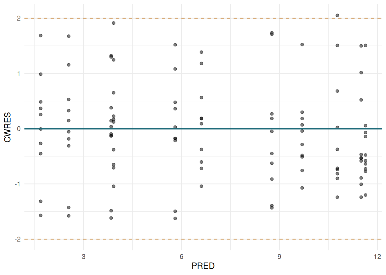
CWRES vs TIME
ggplot(sdtab, aes(x = TIME, y = CWRES)) +
  geom_point(alpha = 0.5) +
  geom_hline(yintercept = 0,      colour = "#1F6B7A", linewidth = 1) +
  geom_hline(yintercept = c(-2, 2), linetype = "dashed", colour = "#C8893E") +
  labs(x = "TIME (h)", y = "CWRES") +
  theme_minimal()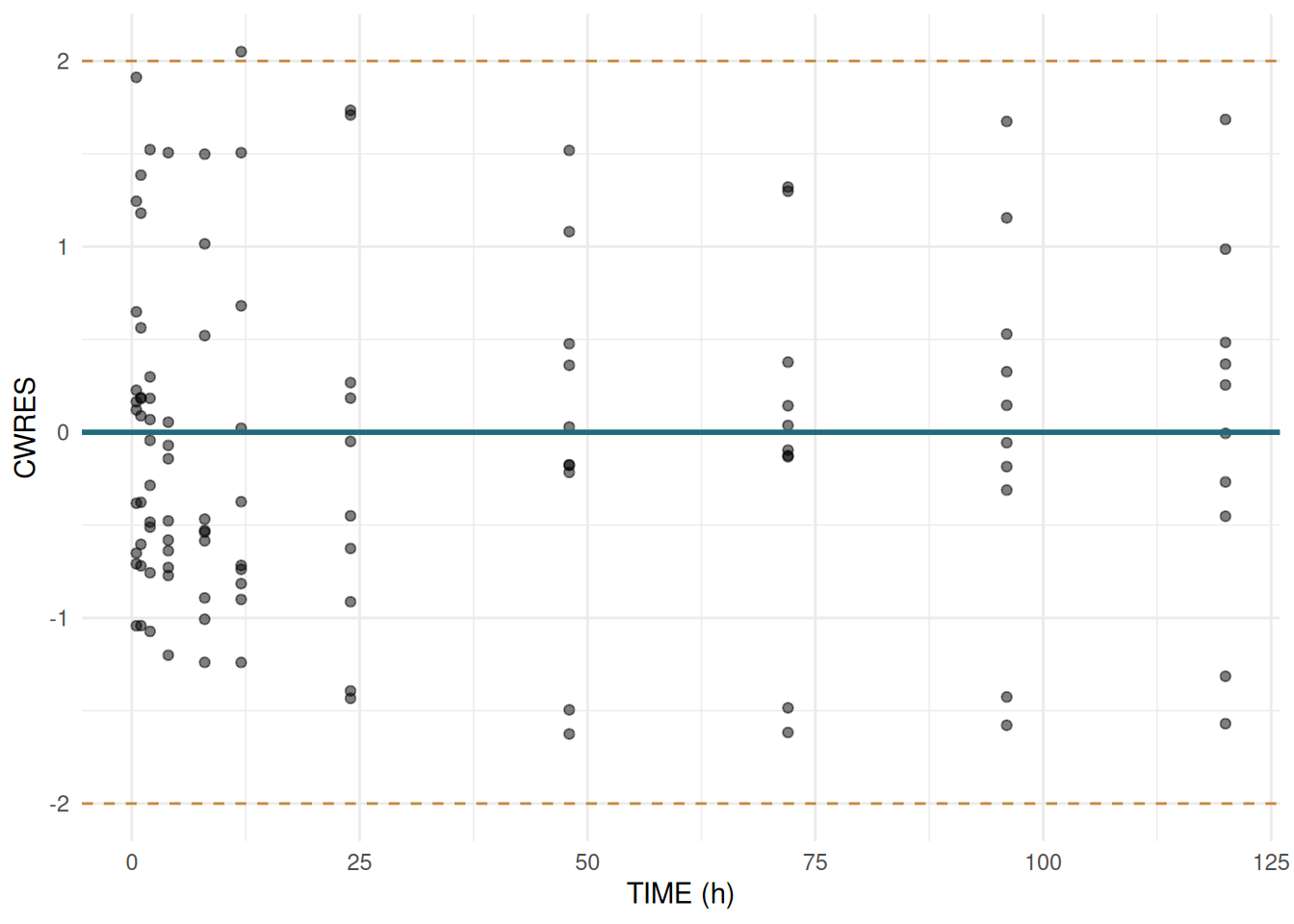
PRED vs DV
ggplot(sdtab, aes(x = PRED, y = DV)) +
  geom_point(alpha = 0.5) +
  geom_abline(slope = 1, intercept = 0, colour = "#1F6B7A", linewidth = 1) +
  labs(x = "PRED", y = "Observed DV") +
  theme_minimal()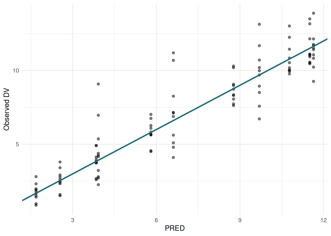
ETA shrinkage
Shrinkage measures how much the individual ETAs are pulled toward zero relative to the omega variance. High shrinkage (> 30%) means the data are not informative enough to reliably estimate individual deviations, and ETA-based diagnostics become unreliable.
fit$shrinkage_eta[1] -0.009554768 0.001434113 0.007254038(summary(fit) also prints shrinkage in its header block.)
ETA shrinkage > 0.3 is a warning sign. It does not mean the model is wrong, but ETA-based covariate plots and individual parameter histograms should be interpreted cautiously.
ETA distribution
ETAs should be approximately normally distributed around zero. Per-subject EBEs are stored in fit$ebe_etas (one row per subject).
etas_long <- fit$ebe_etas |>
  tidyr::pivot_longer(-ID, names_to = "eta", values_to = "value")

ggplot(etas_long, aes(x = value)) +
  geom_histogram(bins = 20, fill = "#1F6B7A", alpha = 0.7) +
  facet_wrap(~eta, scales = "free") +
  labs(x = "EBE", y = "Count") +
  theme_minimal()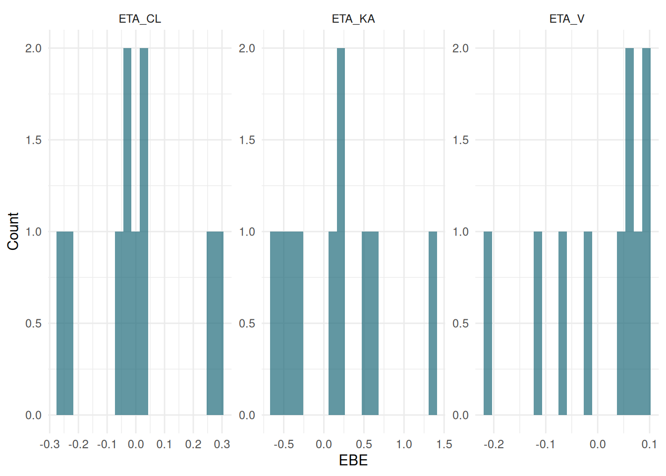
ETA-covariate correlations
ferx_eta_cov() computes Pearson correlations between ETAs and subject-level covariates. The dataset must include numeric covariate columns (the warfarin example has none, so we switch to two_cpt_oral_cov, which carries WT and CRCL):
ex_cov  <- ferx_example("two_cpt_oral_cov")
fit_cov <- ferx_fit(ex_cov$model, ex_cov$data, verbose = FALSE)
Mu-referencing detected for: ETA_CL, ETA_KA, ETA_Q, ETA_V1, ETA_V2ferx_eta_cov(fit_cov, read.csv(ex_cov$data)) eta covariate r p_val flag
1 ETA_KA WT 0.142 0.4546
2 ETA_Q WT 0.108 0.5715
3 ETA_V2 CRCL 0.083 0.6612
4 ETA_CL CRCL 0.077 0.6861
5 ETA_V2 WT 0.073 0.7028
6 ETA_CL WT 0.058 0.7623
7 ETA_Q CRCL 0.043 0.8208
8 ETA_V1 WT -0.011 0.9520
9 ETA_V1 CRCL 0.006 0.9740
10 ETA_KA CRCL -0.002 0.9934 ferx_eta_cov() flags candidates for a covariate search at |r| ≥ 0.3.
Informal covariate screen
ferx_cov_screen(fit) is a broader, informal screen built on the fit’s covariate table (fit$covtab, populated when the model declares a [covariates] block). For every declared covariate it reports the association with each parameter that has IIV, measured two ways: against the subject’s individual parameter estimate (ebe) and against the parameter’s ETA (eta). Covariates are first aggregated to one value per subject – the median for continuous covariates, the most-frequent level for categorical ones. The association is a signed Pearson correlation for continuous covariates and a correlation ratio for categorical covariates; pairs are kept only when an association clears threshold (default |r| ≥ 0.2).
This is a screening aid to decide what is worth a formal covariate search – it is not itself a covariate test or hypothesis test.
ferx_cov_screen(fit_cov, threshold = 0.2)Parameter correlation matrix
After a covariance step, inspect correlations between estimated parameters. Off-diagonal values near ±1 indicate structural identifiability problems.
if (identical(fit$covariance_status, "computed")) {
  ferx_cor_matrix(fit)
} else {
  message("Covariance step did not produce a usable matrix (status: ",
          fit$covariance_status, ").")
}
TVCL TVV TVKA ETA_CL ETA_V ETA_KA PROP_ERR
TVCL 1.000 0.088 -0.089 0.013 0.000 0.021 0.344
TVV 0.088 1.000 0.054 0.002 -0.007 -0.013 0.173
TVKA -0.089 0.054 1.000 -0.001 -0.001 -0.238 -0.238
ETA_CL 0.013 0.002 -0.001 1.000 0.000 0.000 0.004
ETA_V 0.000 -0.007 -0.001 0.000 1.000 0.000 -0.002
ETA_KA 0.021 -0.013 -0.238 0.000 0.000 1.000 0.056
PROP_ERR 0.344 0.173 -0.238 0.004 -0.002 0.056 1.000Parameter estimates table
ferx_estimates() returns a tidy data frame for programmatic use or table export:
ferx_estimates(fit) param transform estimate se rse_pct lower_95
1 TVCL identity 0.132916982 0.0065671817 4.940815 0.120045306
2 TVV identity 7.732457150 0.2341613936 3.028292 7.273500819
3 TVKA identity 0.725734726 0.1250126205 17.225663 0.480709990
4 ETA_CL variance 0.028033006 0.0124211139 44.308890 0.003687623
5 ETA_V variance 0.009584039 0.0043011287 44.878038 0.001153827
6 ETA_KA variance 0.352799315 0.1634646531 46.333608 0.032408595
7 PROP_ERR proportional 0.010717931 0.0009362814 8.735654 0.008882820
upper_95 estimate_natural lower_95_natural upper_95_natural init_as_sd
1 0.14578866 NA NA NA FALSE
2 8.19141348 NA NA NA FALSE
3 0.97075946 NA NA NA FALSE
4 0.05237839 NA NA NA FALSE
5 0.01801425 NA NA NA FALSE
6 0.67319004 NA NA NA FALSE
7 0.01255304 NA NA NA TRUEEpsilon shrinkage
Epsilon shrinkage measures compression in the residual distribution:
fit$shrinkage_eps[1] 0.159018Low epsilon shrinkage (< 20%) is generally acceptable.
IWRES autocorrelation (check_diagnostics)
Residual autocorrelation — IWRES values within a subject that are systematically positive then negative (or vice versa) — is a sign that the structural model is missing dynamics. ferx quantifies this with two pooled statistics computed across all subjects:
| Statistic | Meaning |
|---|---|
| Durbin-Watson (DW) | 2 = no autocorrelation; < 1.5 = positive; > 2.5 = negative |
| Lag-1 Pearson r | Direction and magnitude of serial correlation |
check_diagnostics() returns both in a tidy list alongside shrinkage:
diag <- check_diagnostics(fit)
diag$autocorrelation
dw_statistic lag1_r flag
1 2.608853 -0.3651476 negative autocorrelationdiag$shrinkage param type shrinkage shrinkage_pct
1 ETA_CL eta -0.009554768 -0.9554768
2 ETA_V eta 0.001434113 0.1434113
3 ETA_KA eta 0.007254038 0.7254038
4 PROP_ERR eps 0.159018019 15.9018019print(fit) shows the same values in its DIAGNOSTICS section (one compact line: Covariance: computed Cond: 6.7 DW: 2.61 [negative autocorrelation] IWRES lag-1 r: -0.365), and a message() is emitted automatically when DW < 1.5 or DW > 2.5 with ordered remedies.
Interpreting the DW statistic
| DW range | Interpretation | Suggested action |
|---|---|---|
| < 1.5 | Positive autocorrelation | Check time ordering; add transit compartment; consider IOV on ka/F; SDE |
| 1.5 – 2.5 | No concern | — |
| > 2.5 | Negative autocorrelation | Check for over-parameterisation or misspecified error model |
IWRES vs time plot
if (!is.null(diag$autocorrelation)) {
  dw_val <- diag$autocorrelation$dw_statistic
  r_val  <- diag$autocorrelation$lag1_r
  ggplot(sdtab, aes(x = TIME, y = IWRES, colour = factor(ID))) +
    geom_point(alpha = 0.6, size = 1.5) +
    geom_hline(yintercept = 0, colour = "#1F6B7A", linewidth = 1) +
    labs(
      x = "TIME (h)", y = "IWRES", colour = "Subject",
      title = sprintf("IWRES vs Time  |  DW = %.2f  lag-1 r = %.3f", dw_val, r_val)
    ) +
    theme_minimal() +
    theme(legend.position = "none")
}
Fit warnings (ferx_warnings)
print(fit) ends with a colour-coded warning-count footer (e.g. 1 warning 2 info -- call ferx_warnings(fit) for details). Call ferx_warnings(fit) to see the full grouped output with per-category remediation guidance:
ferx_warnings(fit)Warnings are grouped by severity:
| Severity | Meaning |
|---|---|
critical |
Convergence or covariance failure — results may be unreliable |
warning |
Something worth investigating (e.g. autocorrelation, high %RSE) |
info |
Informational (e.g. mu-referencing detected, thread-pool sizing) |
For programmatic use, ferx_warnings(fit, as_df = TRUE) returns the underlying data frame with columns severity, category, message, and source_method:
ferx_warnings(fit, as_df = TRUE)Run log — ferx_runlog()
ferx_runlog() prints a NONMEM-style .lst summary of a completed fit. It is useful for archiving runs, spotting convergence problems at a glance, and sharing results with colleagues who expect a NONMEM-style output.
ferx_runlog(fit)The output contains these sections (those that depend on optional fields are silently omitted when the fields are absent, so the function degrades gracefully on older .fitrx bundles):
| Section | Contents |
|---|---|
| Run header | Model name, estimation method, ferx version, timestamp |
| Model file | Verbatim content of the .ferx file |
| Data summary | Subject count, observation count, time range |
| Parameter estimates | INITIAL / FINAL / SE / %RSE for every theta, omega, and sigma |
| Estimation settings | Optimizer, max iterations, BLOQ method, NCA warm-start, seeds, covariate columns |
| Objective function | OFV, AIC, BIC, convergence flag |
| Covariance step | Condition number and eigenvalues (requires covariance = TRUE) |
| Diagnostics | ETA/EPS shrinkage, Durbin-Watson, Shapiro-Wilk normality |
| Final gradient | Convergence check for gradient-based optimizers; N/A for BOBYQA/GN/SAEM |
| Runtime | Wall time, gradient methods used |
To capture the output as a string (e.g. for writing to a file):
log_text <- ferx_runlog(fit, verbose = FALSE)
writeLines(log_text, "warfarin_run1.log")
The gradient_tol argument (default 0.01) controls the threshold for flagging individual gradient components as non-converged:
ferx_runlog(fit, gradient_tol = 0.001) # stricter than the defaultCovariance condition number
After the covariance step, fit$condition_number gives the ratio of the largest to smallest eigenvalue of the correlation matrix of estimates. It is shown in print(fit) and summary(fit) as Cond: <value>.
| Condition number | Interpretation |
|---|---|
| < 100 | Well-conditioned; estimates are stable |
| 100 – 1000 | Mild ill-conditioning; inspect high-correlation parameter pairs |
| > 1000 | Severe ill-conditioning; ferx emits a warning. Consider removing parameters or re-parameterising |
Inf |
Non-positive eigenvalue — covariance matrix is singular |
fit$condition_number
fit$eigenvalues      # full sorted vector; the ratio of first to last is condition_number
ferx_cor_matrix(fit) shows the off-diagonal parameter correlations that drive a high condition number — pairs near ±1 are the culprits.