library(ferx)
ex <- ferx_example("warfarin")Fitting
Overview
ferx_fit() is the central function. It compiles the model, runs the optimiser, and returns a ferx_fit object with estimates, standard errors, and individual diagnostics.
Estimation methods
A fit has two layers that are worth keeping distinct from the start:
- the method (
foce,focei,saem,gn,gn_hybrid,imp) decides what objective is maximised — how the likelihood integrates over the random effects; - the optimizer (
bobyqa,slsqp,trust_region, …) decides how that objective is minimised over the parameter vector.
Not every optimizer applies to every method, and each method has its own tuning knobs. The Optimizer and method settings section below lays out the full grid; this section covers the method choice itself.
Pass method to choose the algorithm:
| Method | Description | Typical use |
|---|---|---|
"foce" |
First-Order Conditional Estimation | Default, fast, well-tested |
"focei" |
FOCE with interaction | When residual error depends on ETAs |
"saem" |
Stochastic Approximation EM | Models with many ETAs or strong nonlinearity; supports IOV |
"gn" |
Gauss-Newton / BHHH | Quick exploration; runs its own loop, no covariance |
"gn_hybrid" |
Gauss-Newton then FOCEI polish | Fast warm start, rigorous finish |
"imp" |
Importance-sampling marginal log-likelihood | Standalone scoring of initial parameters, or as the terminal stage of a chain; see Overview |
fit_foce <- ferx_fit(ex$model, ex$data, method = "foce")Mu-referencing detected for: ETA_CL, ETA_KA, ETA_Vfit_focei <- ferx_fit(ex$model, ex$data, method = "focei")Warning: Model file [fit_options] sets `method = foce` but ferx_fit() argument
overrides it with `focei`. The call-time value will be used.Mu-referencing detected for: ETA_CL, ETA_KA, ETA_VMethod chains
Pass a character vector to run methods in sequence. Each stage is seeded with the previous stage’s converged parameters. Only the final stage produces the reported covariance and diagnostics.
A common production pattern is c("saem", "focei") — SAEM finds the basin of attraction robustly, FOCEI polishes and produces the covariance step. A second useful chain is c("focei", "imp"): the final imp stage runs importance sampling around the FOCEI mode and reports the marginal log-likelihood and effective sample size, which give an honest read on the Laplace approximation. See Overview for the imp diagnostics.
imp can also run standalone (method = "imp") with no preceding estimator, in which case it scores the model file’s initial parameters rather than a converged mode — useful as a cheap likelihood probe of a candidate parameterisation before committing to a full fit:
fit_imp <- ferx_fit(ex$model, ex$data, method = "imp")Pre-fit sanity checks
Two helpers run before the expensive fit and catch most “won’t converge” problems early.
Initial-value check
ferx_check_init() runs a handful of optimiser iterations from the model file’s initial estimates and returns a list with a $trace data frame (per- iteration OFV, gradient norm, step norm) and a $summary row (start OFV, end OFV, OFV drop, convergence flag). A finite start OFV and a non-degenerate gradient mean the model is set up correctly enough to attempt the full fit; a non-finite OFV or an explosive gradient norm flags scale or specification problems before you commit to a long run.
ferx_check_init(ex$model, ex$data)Inspecting the data columns
ferx_columns() reads only the header row of a NONMEM-format CSV and prints the column names grouped into required NONMEM columns (ID, TIME, DV, EVID, AMT, CMT), optional NONMEM columns (RATE, MDV, II, SS, CENS, OCC), and covariates / user-defined columns. It is a fast way to confirm the dataset has the columns the model expects before fitting. It accepts a path, a ferx_fit object, or the list returned by ferx_example():
ferx_columns(ex)        # pass the ferx_example() list directly
ferx_columns(ex$data)   # or pass the path
NCA-based initial estimates
If you do not have good initial estimates, ferx_inits_from_nca() derives them from a per-subject non-compartmental analysis and returns starting theta and omega values:
inits <- ferx_inits_from_nca(ex$model, ex$data, method = "nca")
inits$theta
inits$omega
The same routine is also available inside ferx_fit() via the inits_from_nca argument; pass "nca", "nca_sweep" (default when inits_from_nca = TRUE), or "nca_ebe" to swap initial values in automatically.
The covariance step
covariance = TRUE triggers the Hessian-based covariance matrix after convergence. This provides standard errors, 95% confidence intervals, and the condition number.
fit <- ferx_fit(ex$model, ex$data, method = "foce", covariance = TRUE,
                optimizer_trace = TRUE, verbose = FALSE)
Mu-referencing detected for: ETA_CL, ETA_KA, ETA_VAfter convergence inspect fit$covariance_status:
-
"computed"— Hessian is positive-definite; SEs and 95% CIs are available inferx_estimates(fit). -
"sir_fallback"— the finite-difference Hessian was not positive-definite, butcovariance_fallback = "sir"ran SIR with an absolute-eigenvalue-rectified proposal and reported SIR-based intervals instead of failing (see below). -
"failed"— covariance matrix could not be inverted or was non-positive-definite.fit$cov_matrixand these/CI columns areNA. Likely causes are over-parameterisation, a boundary estimate, or a parameter that is structurally non-identifiable. -
"not_requested"— the fit ran withcovariance = FALSE, so no covariance step was attempted.
When the covariance step fails, ferx does not just say “failed”: the warning on fit$warnings carries failure-mode-specific guidance, and the exact advice depends on why the Hessian was unusable. The cases it distinguishes are:
- Omega near-singular (“omega matrix is not positive definite”) — suggests a diagonal omega, fixing a small variance to a small positive constant, or dropping the corresponding ETA.
- Non-PD Hessian with an eigenvalue list — points you at the printed eigenvalues: a near-zero minimum flags a near-unidentifiable parameter, a clearly negative minimum flags structural non-identifiability.
-
Ill-conditioned entries (flat or non-finite Hessian diagonal for named parameters) — suggests fixing the parameter, tightening its bounds, or raising
fd_hessian_step(see below). - Non-finite base OFV — model evaluation overflowed/underflowed at convergence; check for extreme parameter values and that DV is positive under proportional error.
-
Regularisation applied — graded by severity (minor / moderate / severe); severe means SEs are likely unreliable and you should cross-check with
ferx_sir().
Switching to SAEM, which does not depend on the Hessian for convergence, is a robust last resort when the structural model itself is the problem.
Covariance-robustness controls
Three ferx_fit() arguments tune the covariance step itself when the default inverse-Hessian computation is fragile:
-
fd_hessian_step(default0.01) — relative step size for the finite-difference Hessian; the actual perturbation for parameter i isfd_hessian_step * (1 + |x_hat[i]|). Raise it (e.g.0.05) when the fit warns about ill-conditioned Hessian entries; lower it (e.g.1e-3) on smooth surfaces where finite-difference noise dominates. No effect whencovariance = FALSE. -
covariance_method— the estimator, mirroring NONMEM$COV MATRIX=:"r"(inverse Hessian, the default),"s"(score cross-product), or"rsr"(the Huber-White sandwich, robust to model misspecification)."s"and"rsr"are rejected under non-interaction FOCE — use FOCEI for those. Passed viasettings. -
covariance_fallback—"none"(default) or"sir". When the finite-difference Hessian is not positive-definite,"sir"runs SIR with an absolute-eigenvalue-rectified proposal instead of leaving the step failed;covariance_statusthen becomes"sir_fallback"and SIR-based credible intervals are reported. Passed viasettings.
fd_hessian_step is a dedicated top-level argument; covariance_method and covariance_fallback are passed through settings:
Parallelism
ferx uses parallelism at two independent levels. Understanding both helps you get the most out of a multi-core machine.
Per-subject parallelism (threads)
The inner loops run in parallel across subjects on threads workers. This applies to all estimation methods:
| Method | What is parallelised |
|---|---|
| FOCE / FOCEI | EBE (inner) optimisation per subject |
| SAEM | Metropolis-Hastings sampling per subject |
| GN / GN hybrid | Per-subject gradient evaluations |
fit <- ferx_fit(ex$model, ex$data, threads = parallel::detectCores(logical = FALSE))Passing NULL (the default) uses one worker per logical CPU. On HPC shared nodes, cap the thread count to avoid contention:
fit <- ferx_fit(ex$model, ex$data, threads = 4L)This speeds up a single fit by distributing subjects across cores. It does not help when the model is stuck in a local minimum.
threads controls the inner-loop pool only. The n_starts outer parallelism (see below) always uses the global rayon pool regardless of threads.
Multi-start optimization (n_starts)
Some models have multimodal OFV surfaces where a single fit can converge to a local minimum rather than the global optimum. This is common with:
- Michaelis-Menten (saturable) elimination — the Vmax/Km pair produces a narrow ridge where many combinations give similar predicted concentrations.
- Full-block omega with three or more ETAs.
- Many correlated covariate parameters.
n_starts runs independent fits from perturbed starting values in parallel and returns the result with the lowest OFV:
The default is n_starts = 1, which runs a single fit with no perturbation — multi-start is opt-in. With n_starts = 8, the first run (internally labelled start 0) uses the exact initial values from the model file; starts 1–7 apply a log-space perturbation of size start_sigma (default 0.3, roughly ±30% CV) to each theta. Setting n_starts = 0 is rejected at parse time with an error. On an 8-core machine, 8 starts cost approximately the same wall time as a single run.
For ridge-shaped surfaces — where the optimiser needs to explore a wider neighbourhood — increase start_sigma:
Pin multi_start_seed to reproduce a specific set of perturbations:
Method and optimizer behaviour:
| Method | Multi-start behaviour |
|---|---|
| FOCE / FOCEI | Fully supported; most useful — gradient-based methods are most prone to local minima |
| GN / GN hybrid | Fully supported; same local-minimum risk as FOCE |
| SAEM | Supported; each start gets an independent MH sampler seed (saem_seed + k) so trajectories are stochastically distinct. SAEM is inherently more robust to local minima than FOCE, but multi-start still helps on very multimodal surfaces |
n_starts is optimizer-agnostic: it works with any optimizer setting (slsqp, bobyqa, trust_region, lbfgs, etc.) — each start runs the full local optimisation pipeline with its own perturbed theta.
Warning
global_search interaction: when global_search = true and n_starts > 1, the CRS2-LM gradient-free pre-search only runs on start 0. CRS2-LM ignores the starting point by design, so running it on perturbed starts would override the perturbation and waste cores. ferx emits a warning on fit$warnings when this combination is detected.
Combining both levels
threads and n_starts are orthogonal and compose naturally. With n_starts = 4 and threads = 2, ferx runs four fits in parallel, each using two worker threads for its inner loops — fully utilizing an 8-core machine:
Tip
Rule of thumb: use threads to speed up a single well-conditioned fit; use n_starts when you suspect local minima. On a shared HPC node where you have 8 cores, n_starts = 8, threads = 1 is usually better than n_starts = 1, threads = 8 for poorly-identified models.
Optimizer and method settings
Everything beyond the dedicated ferx_fit() arguments is tuned through the settings list (or, equivalently, the model file’s [fit_options] block). Keys are validated — an unknown key, a malformed value, or a key that duplicates a dedicated argument (method, covariance, bloq_method, threads, sir) raises an error rather than being silently ignored.
Precedence. Dedicated arguments win over settings, which win over the model file’s [fit_options]. A warning() fires whenever a call-time value overrides a different value baked into the model file. Inspect fit$call_settings and fit$model_file_settings to audit what actually took effect.
Which settings apply to which method
The single most common source of confusion is passing an option to a method that ignores it. This grid is the map:
| Setting | FOCE / FOCEI | GN-hybrid | pure GN | SAEM | IMP stage |
|---|---|---|---|---|---|
optimizer |
✓ | polish only | — | — | — |
maxiter |
✓ | ✓ | ✓ | — (use n_*) |
— |
global_search, global_maxeval
|
✓ | polish only | — | — | — |
stagnation_guard |
✓ | ✓ | — | — | — |
reconverge_gradient_interval |
✓ | ✓ | — | — | — |
steihaug_max_iters (trust-region) |
✓ | ✓ | — | — | — |
gn_lambda |
— | ✓ | ✓ | — | — |
n_exploration, n_convergence, n_mh_steps, adapt_interval, omega_burnin, n_leapfrog
|
— | — | — | ✓ | — |
is_samples, is_proposal_df, is_seed, is_low_ess_threshold
|
— | — | — | — | ✓ |
inner_maxiter, inner_tol (shared) |
✓ | ✓ | ✓ | ✓ | — |
Setting an option that the active method ignores is harmless for most keys but optimizer under method = "saem" emits a warning — SAEM has no single outer minimisation, so there is no algorithm to select.
The outer optimizer
For FOCE / FOCEI (and the FOCEI polish phase of gn_hybrid), the outer optimizer minimises the population OFV over the transformed parameter vector [log θ, chol(Ω), log σ]:
| Optimizer | Kind | Use it when |
|---|---|---|
bobyqa (default)
|
Derivative-free quadratic trust-region | Start here. Re-evaluates the EBEs at every trial point, so it never sees the fixed-EBE gradient bias that stalls gradient methods on ODE/PD models, sparse data, and Hill-ridge identifiability problems. |
slsqp |
Gradient-based SQP | A smooth, well-conditioned analytical-PK model with many parameters, where derivative-free search needs too many samples to triangulate the surface. |
trust_region |
Newton trust-region (Steihaug CG) | Large θ + Ω, or paired with inits_from_nca (see NCA-based initial estimates) — second-order curvature helps when you are already in the right basin. |
lbfgs, nlopt_lbfgs, mma, bfgs
|
Quasi-Newton / SQP variants | Rarely needed; prefer bobyqa or slsqp. |
NoteWhy
bobyqa is the default
The default was slsqp in earlier releases. On ODE/PD models and sparse data, the cheap fixed-EBE finite-difference gradient drives slsqp to local minima hundreds of OFV units above the true optimum. bobyqa doesn’t use a gradient, doesn’t see the bias, and reaches the same or lower OFV in the same or less wall time. Pure gn and pure saem ignore optimizer entirely.
Fixed-EBE gradient bias and reconverge_gradient_interval
This is the knob behind the default change, and the first thing to reach for when a gradient-based optimizer stalls above an OFV you expected to beat.
By default (reconverge_gradient_interval = 0) the population gradient holds each subject’s inner EBE solution fixed — cheap, but it omits the response of that inner solution to θ and Ω. On ill-conditioned non-IOV models the omitted term is exactly what lets slsqp stall. Reconverging the inner loop during the gradient recovers the full surface at roughly 5–6× the per-gradient cost:
-
0— never reconverge (cheap fixed-EBE gradient, the default); -
1— reconverge on every gradient evaluation (full surface, full cost); -
N— reconverge everyN-th evaluation, cheap gradient in between, which often closes most of the gap for a fraction of the cost.
IOV models always reconverge and ignore this setting.
Letting the optimizer run: stagnation_guard
By default ferx short-circuits the NLopt outer loop once the OFV plateau is numerically flat (no improvement above 1e-3 over a rolling window), so SLSQP / L-BFGS terminate quickly instead of grinding through the full maxiter budget at full inner-loop cost. Set stagnation_guard = FALSE to disable the guard and let the optimizer run to its own xtol / ftol or to maxiter — useful when real OFV improvements are genuinely smaller than the guard’s threshold (some γ-bearing FOCEI problems), or when debugging.
Global pre-search
global_search = TRUE runs NLopt’s CRS2-LM derivative-free search to find a good basin before the local optimizer takes over — useful when initial estimates are weak (e.g. translated from a different drug) and you would rather not spend a full SAEM stage. It requires lower/upper bounds on every theta and hands off to the optimizer once global_maxeval is exhausted.
Combine with n_starts (see Multi-start optimization) only when you understand the interaction described in that section’s warning.
SAEM-specific settings
SAEM controls its own iteration budget instead of maxiter, and exposes the sampler internals:
| Setting | Default | What it does |
|---|---|---|
n_exploration |
150 | Stochastic exploration-phase iterations. |
n_convergence |
250 | Averaging / convergence-phase iterations. |
n_mh_steps |
3 | Metropolis-Hastings steps per subject per iteration. |
adapt_interval |
50 | How often (iterations) the MH proposal covariance is adapted. |
omega_burnin |
20 | Iterations holding Ω fixed while the sampler warms up. Guards against Ω collapse on sparse data; set 0 to disable. |
seed / saem_seed
|
12345 | RNG seed for the MH sampler. |
n_leapfrog / saem_n_leapfrog
|
0 |
0 = Metropolis-Hastings; a positive value swaps in one HMC proposal per subject per iteration. |
If your SAEM fit on sparse data shows a tiny omega paired with an inflated additive sigma, raise omega_burnin before anything else — that pattern is the classic Ω-collapse the burn-in is there to prevent.
Gauss-Newton, IMP and SIR settings
| Setting | Applies to | Default | What it does |
|---|---|---|---|
gn_lambda |
gn, gn_hybrid
|
0.01 | Levenberg-Marquardt damping; larger = more conservative steps. |
steihaug_max_iters |
trust_region |
engine | CG iteration budget for the trust-region subproblem; raise on ill-conditioned problems. |
is_samples |
imp stage |
1000 | Importance samples per subject (halving the MC SE needs 4× the samples). |
is_proposal_df |
imp stage |
5 | Degrees of freedom for the Student-t proposal. |
is_seed |
imp stage |
engine | RNG seed for the importance-sampling step. |
is_low_ess_threshold |
imp stage |
0.1 | ESS fraction below which a subject is flagged. |
For the SIR (sir_samples, sir_resamples, sir_seed) and multi-start (n_starts, start_sigma, multi_start_seed) knobs, see Overview and Multi-start optimization respectively — they have dedicated sections rather than being repeated here.
Reading the output
summary(fit)--------------------------------------------------
ferx NLME Fit Summary
--------------------------------------------------
Model: warfarin
Dataset: warfarin
Converged: YES
Method: FOCE
Gradient: auto (requested) -> analytic (Dual2) (used)
ferx v0.1.6 (core v0.1.6)
Settings (model file / call-time override):
method foce [model only]
maxiter 300 [model only]
covariance true [model only]
optimizer_trace TRUE
Structure: 1-cpt oral (TVCL, TVV, TVKA) | IIV: ETA_CL, ETA_V, ETA_KA | IOV: none | Residual: proportional
OFV: -280.3601 AIC: -266.3601 BIC: -247.4567
Subjects: 10 Obs: 110 Params: 7 Iter: 57
Shrinkage: ETA1=-1.0% ETA2=0.1% ETA3=0.7%
EPS shrinkage: 15.9%
DW: 2.61 [negative autocorrelation]
lag-1 r: -0.365
Covariance: computed Cond: 2.6 | Wall time: 0.3s
Warnings:
* mu-ref: ETA_CL, ETA_KA, ETA_V
* Negative IWRES autocorrelation detected (Durbin-Watson = 2.61). Possible over-parameterization or misspecified error model.
* 28 EBE fallback(s)
--------------------------------------------------summary(fit) is the run report: convergence, method, OFV/AIC/BIC, auto-derived model structure, shrinkage, DW statistic, gradient method requested vs used, covariance status and condition number, wall time, and warnings. The parameter table itself (THETA / OMEGA / SIGMA point estimates + SE) is shown by print(fit) or as a tidy data frame by ferx_estimates(fit).
Accessing individual fields
fit$theta # named numeric vector of theta estimates TVCL TVV TVKA
0.1329170 7.7324572 0.7257347 fit$omega # omega matrix ETA_CL ETA_V ETA_KA
ETA_CL 0.02803301 0.000000000 0.0000000
ETA_V 0.00000000 0.009584039 0.0000000
ETA_KA 0.00000000 0.000000000 0.3527993fit$sigma # sigma vector[1] 0.01071793fit$se_theta # SEs for theta TVCL TVV TVKA
0.006567182 0.234161394 0.125012620 fit$ofv # scalar OFV[1] -280.3601fit$aic[1] -266.3601fit$bic[1] -247.4567fit$sdtab # individual-level diagnostics (ID, TIME, DV, PRED, IPRED, CWRES, ...) ID TIME DV PRED IPRED CWRES IWRES EBE_OFV
1 1 0.5 5.3653 3.917754 5.3517714 0.648955031 0.235855380 -27.11921
2 1 1.0 8.2578 6.609725 8.2834304 0.562551563 -0.288692038 -27.11921
3 1 2.0 10.7063 9.695979 10.7084507 0.298277847 -0.018738589 -27.11921
4 1 4.0 11.4142 11.639355 11.3832622 -0.477260194 0.253577856 -27.11921
5 1 8.0 10.9232 11.504506 10.7577615 -0.584560380 1.434840567 -27.11921
6 1 12.0 9.9442 10.775094 10.0692822 -0.900618045 -1.159007239 -27.11921
7 1 24.0 8.0634 8.768506 8.2547844 -0.913245374 -2.163166171 -27.11921
8 1 48.0 5.6575 5.804414 5.5477818 -0.177647532 1.845220826 -27.11921
9 1 72.0 3.7373 3.842299 3.7284902 -0.132016291 0.220455882 -27.11921
10 1 96.0 2.5019 2.543455 2.5058014 -0.056470504 -0.145264515 -27.11921
11 1 120.0 1.6785 1.683669 1.6840705 -0.006189828 -0.308621240 -27.11921
12 2 0.5 3.2230 3.917754 3.2273948 -0.382052390 -0.127051616 -33.20136
13 2 1.0 5.6205 6.609725 5.6653473 -0.377098394 -0.738582352 -33.20136
14 2 2.0 8.9389 9.695979 8.8734083 -0.286109560 0.688628506 -33.20136
15 2 4.0 11.6945 11.639355 11.5827999 -0.070644098 0.899764744 -33.20136
16 2 8.0 12.1458 11.504506 12.1057407 0.520591556 0.308745745 -33.20136
17 2 12.0 11.4394 10.775094 11.3956592 0.681257687 0.358126635 -33.20136
18 2 24.0 8.9787 8.768506 9.1334277 0.267467463 -1.580604429 -33.20136
19 2 48.0 5.8306 5.804414 5.8437599 0.028338130 -0.210111448 -33.20136
20 2 72.0 3.7432 3.842299 3.7389461 -0.125699515 0.106151245 -33.20136
21 2 96.0 2.4121 2.543455 2.3922472 -0.185038510 0.774293340 -33.20136
22 2 120.0 1.5248 1.683669 1.5306042 -0.267735716 -0.353806482 -33.20136
23 3 0.5 4.3905 3.917754 4.4258975 0.226430012 -0.746209270 -31.45602
24 3 1.0 7.1595 6.609725 7.1525291 0.186961959 0.090932221 -31.45602
25 3 2.0 9.9835 9.695979 9.8260759 0.068369416 1.494789489 -31.45602
26 3 4.0 11.0602 11.639355 11.0164082 -0.580824027 0.370887242 -31.45602
27 3 8.0 10.5157 11.504506 10.6138100 -1.007220546 -0.862444242 -31.45602
28 3 12.0 10.0334 10.775094 9.9886795 -0.815358643 0.417722520 -31.45602
29 3 24.0 8.3092 8.768506 8.3113411 -0.625717143 -0.024035179 -31.45602
30 3 48.0 5.6709 5.804414 5.7541957 -0.216005471 -1.350600751 -31.45602
31 3 72.0 3.9685 3.842299 3.9838057 0.142875613 -0.358463455 -31.45602
32 3 96.0 2.7817 2.543455 2.7581106 0.326002650 0.797984551 -31.45602
33 3 120.0 1.9121 1.683669 1.9095243 0.367150899 0.125849635 -31.45602
34 4 0.5 2.8040 3.917754 2.8204821 -0.651032739 -0.545226551 -30.59908
35 4 1.0 5.0987 6.609725 5.1115153 -0.603611638 -0.233919789 -30.59908
36 4 2.0 8.5069 9.695979 8.4654946 -0.484249187 0.456345848 -30.59908
37 4 4.0 12.1373 11.639355 11.9984185 -0.142728075 1.079964190 -30.59908
38 4 8.0 13.4967 11.504506 13.5618672 1.014898268 -0.448330860 -30.59908
39 4 12.0 13.0143 10.775094 13.0139208 2.050141018 0.002718295 -30.59908
40 4 24.0 10.3014 8.768506 10.2781374 1.708954806 0.211170076 -30.59908
41 4 48.0 6.2732 5.804414 6.2633470 0.476580509 0.146774285 -30.59908
42 4 72.0 3.7865 3.842299 3.8162619 -0.096112026 -0.727631702 -30.59908
43 4 96.0 2.3290 2.543455 2.3252511 -0.311504321 0.150425405 -30.59908
44 4 120.0 1.4205 1.683669 1.4167772 -0.452489034 0.245166114 -30.59908
45 5 0.5 6.9670 3.917754 6.9964305 1.244430833 -0.392473708 -24.51315
46 5 1.0 10.6865 6.609725 10.5738280 1.385083106 0.994197967 -24.51315
47 5 2.0 13.1310 9.695979 13.2604492 1.522463637 -0.910815209 -24.51315
48 5 4.0 13.8818 11.639355 13.8210176 1.505995521 0.410323614 -24.51315
49 5 8.0 13.1620 11.504506 13.0698003 1.497954435 0.658187546 -24.51315
50 5 12.0 12.2496 10.775094 12.2910240 1.505948368 -0.314451282 -24.51315
51 5 24.0 10.1919 8.768506 10.2212716 1.734457508 -0.268109105 -24.51315
52 5 48.0 7.0234 5.804414 7.0686828 1.518171327 -0.597701343 -24.51315
53 5 72.0 4.9146 3.842299 4.8884600 1.320802894 0.498910722 -24.51315
54 5 96.0 3.4118 2.543455 3.3806922 1.154717703 0.858524314 -24.51315
55 5 120.0 2.3219 1.683669 2.3379714 0.986439824 -0.641363871 -24.51315
56 6 0.5 9.0826 3.917754 9.0673730 1.911655877 0.156683166 -28.00588
57 6 1.0 11.1962 6.609725 11.2101757 1.180203136 -0.116319281 -28.00588
58 6 2.0 11.6818 9.695979 11.7023480 -0.511031886 -0.163827130 -28.00588
59 6 4.0 11.5303 11.639355 11.3784874 -0.638253988 1.244836864 -28.00588
60 6 8.0 10.5567 11.504506 10.6789788 -0.892418872 -1.068342736 -28.00588
61 6 12.0 10.0149 10.775094 10.0223384 -0.738283639 -0.069247117 -28.00588
62 6 24.0 8.3510 8.768506 8.2848963 -0.450132843 0.744436206 -28.00588
63 6 48.0 5.6307 5.804414 5.6613905 -0.175488884 -0.505788811 -28.00588
64 6 72.0 3.8447 3.842299 3.8686473 0.036979698 -0.577545861 -28.00588
65 6 96.0 2.6274 2.543455 2.6435965 0.145232061 -0.571629770 -28.00588
66 6 120.0 1.8242 1.683669 1.8064718 0.254982103 0.915633069 -28.00588
67 7 0.5 2.2639 3.917754 2.2717137 -1.042653720 -0.320918473 -32.81792
68 7 1.0 4.1060 6.609725 4.0919042 -1.041726653 0.321404394 -32.81792
69 7 2.0 6.7205 9.695979 6.7023418 -1.072510196 0.252775376 -32.81792
70 7 4.0 9.2610 11.639355 9.3325834 -1.200788040 -0.715647805 -32.81792
71 7 8.0 10.4566 11.504506 10.3241537 -1.239614765 1.196945729 -32.81792
72 7 12.0 9.7727 10.775094 9.8035688 -1.240019776 -0.293781706 -32.81792
73 7 24.0 7.6251 8.768506 7.6331647 -1.393254945 -0.098576477 -32.81792
74 7 48.0 4.5665 5.804414 4.5480082 -1.495234122 0.379355428 -32.81792
75 7 72.0 2.6819 3.842299 2.7095969 -1.484538632 -0.953708490 -32.81792
76 7 96.0 1.5919 2.543455 1.6143144 -1.426020245 -1.295474387 -32.81792
77 7 120.0 0.9761 1.683669 0.9617708 -1.314284488 1.390081259 -32.81792
78 8 0.5 4.1618 3.917754 4.2214781 0.120888547 -1.318983241 -26.13768
79 8 1.0 7.1196 6.609725 7.0334758 0.181353264 1.142467969 -26.13768
80 8 2.0 10.1932 9.695979 10.1026676 0.182848481 0.836097799 -26.13768
81 8 4.0 11.7577 11.639355 11.7789421 0.054422693 -0.168259617 -26.13768
82 8 8.0 11.1099 11.504506 11.2708660 -0.467939913 -1.332495617 -26.13768
83 8 12.0 10.5284 10.775094 10.3076091 -0.374209902 1.998537199 -26.13768
84 8 24.0 7.7364 8.768506 7.8320046 -1.433156340 -1.138924728 -26.13768
85 8 48.0 4.5075 5.804414 4.5206714 -1.625144546 -0.271842914 -26.13768
86 8 72.0 2.6025 3.842299 2.6093536 -1.617247994 -0.245062084 -26.13768
87 8 96.0 1.5117 2.543455 1.5061317 -1.578323775 0.344946646 -26.13768
88 8 120.0 0.8700 1.683669 0.8693466 -1.569624860 0.070130467 -26.13768
89 9 0.5 4.2570 3.917754 4.2359261 0.164028296 0.464177999 -16.67525
90 9 1.0 6.8848 6.609725 6.9180413 0.088687259 -0.448315171 -16.67525
91 9 2.0 9.6938 9.695979 9.6616452 -0.043464956 0.310515585 -16.67525
92 9 4.0 10.8291 11.639355 11.0443900 -0.728244791 -1.818742515 -16.67525
93 9 8.0 11.0184 11.504506 10.8325485 -0.528886194 1.600753333 -16.67525
94 9 12.0 10.1868 10.775094 10.3315170 -0.717148189 -1.306906375 -16.67525
95 9 24.0 9.0680 8.768506 8.9411539 0.183874078 1.323648146 -16.67525
96 9 48.0 6.7533 5.804414 6.6962369 1.080586663 0.795084406 -16.67525
97 9 72.0 4.9146 3.842299 5.0149667 1.298268085 -1.867285286 -16.67525
98 9 96.0 3.8000 2.543455 3.7558245 1.673963365 1.097399424 -16.67525
99 9 120.0 2.8068 1.683669 2.8128239 1.684930244 -0.199812077 -16.67525
100 10 0.5 2.7113 3.917754 2.6978952 -0.708680312 0.463579498 -29.83454
101 10 1.0 4.7969 6.609725 4.7875953 -0.719394754 0.181331246 -29.83454
102 10 2.0 7.5839 9.695979 7.6437694 -0.756989761 -0.730779372 -29.83454
103 10 4.0 10.2283 11.639355 10.2726036 -0.771771636 -0.402390501 -29.83454
104 10 8.0 11.0856 11.504506 11.0937195 -0.537674558 -0.068287557 -29.83454
105 10 12.0 10.8385 10.775094 10.6261704 0.021891812 1.864329638 -29.83454
106 10 24.0 8.7349 8.768506 8.8447377 -0.049421578 -1.158658504 -29.83454
107 10 48.0 6.0869 5.804414 6.0872202 0.360810374 -0.004907125 -29.83454
108 10 72.0 4.1361 3.842299 4.1893654 0.377688382 -1.186277681 -29.83454
109 10 96.0 2.9208 2.543455 2.8832180 0.528914832 1.216161372 -29.83454
110 10 120.0 1.9807 1.683669 1.9842972 0.484111793 -0.169140552 -29.83454
N_OBS TAFD TAD
1 11 0.5 0.5
2 11 1.0 1.0
3 11 2.0 2.0
4 11 4.0 4.0
5 11 8.0 8.0
6 11 12.0 12.0
7 11 24.0 24.0
8 11 48.0 48.0
9 11 72.0 72.0
10 11 96.0 96.0
11 11 120.0 120.0
12 11 0.5 0.5
13 11 1.0 1.0
14 11 2.0 2.0
15 11 4.0 4.0
16 11 8.0 8.0
17 11 12.0 12.0
18 11 24.0 24.0
19 11 48.0 48.0
20 11 72.0 72.0
21 11 96.0 96.0
22 11 120.0 120.0
23 11 0.5 0.5
24 11 1.0 1.0
25 11 2.0 2.0
26 11 4.0 4.0
27 11 8.0 8.0
28 11 12.0 12.0
29 11 24.0 24.0
30 11 48.0 48.0
31 11 72.0 72.0
32 11 96.0 96.0
33 11 120.0 120.0
34 11 0.5 0.5
35 11 1.0 1.0
36 11 2.0 2.0
37 11 4.0 4.0
38 11 8.0 8.0
39 11 12.0 12.0
40 11 24.0 24.0
41 11 48.0 48.0
42 11 72.0 72.0
43 11 96.0 96.0
44 11 120.0 120.0
45 11 0.5 0.5
46 11 1.0 1.0
47 11 2.0 2.0
48 11 4.0 4.0
49 11 8.0 8.0
50 11 12.0 12.0
51 11 24.0 24.0
52 11 48.0 48.0
53 11 72.0 72.0
54 11 96.0 96.0
55 11 120.0 120.0
56 11 0.5 0.5
57 11 1.0 1.0
58 11 2.0 2.0
59 11 4.0 4.0
60 11 8.0 8.0
61 11 12.0 12.0
62 11 24.0 24.0
63 11 48.0 48.0
64 11 72.0 72.0
65 11 96.0 96.0
66 11 120.0 120.0
67 11 0.5 0.5
68 11 1.0 1.0
69 11 2.0 2.0
70 11 4.0 4.0
71 11 8.0 8.0
72 11 12.0 12.0
73 11 24.0 24.0
74 11 48.0 48.0
75 11 72.0 72.0
76 11 96.0 96.0
77 11 120.0 120.0
78 11 0.5 0.5
79 11 1.0 1.0
80 11 2.0 2.0
81 11 4.0 4.0
82 11 8.0 8.0
83 11 12.0 12.0
84 11 24.0 24.0
85 11 48.0 48.0
86 11 72.0 72.0
87 11 96.0 96.0
88 11 120.0 120.0
89 11 0.5 0.5
90 11 1.0 1.0
91 11 2.0 2.0
92 11 4.0 4.0
93 11 8.0 8.0
94 11 12.0 12.0
95 11 24.0 24.0
96 11 48.0 48.0
97 11 72.0 72.0
98 11 96.0 96.0
99 11 120.0 120.0
100 11 0.5 0.5
101 11 1.0 1.0
102 11 2.0 2.0
103 11 4.0 4.0
104 11 8.0 8.0
105 11 12.0 12.0
106 11 24.0 24.0
107 11 48.0 48.0
108 11 72.0 72.0
109 11 96.0 96.0
110 11 120.0 120.0Convergence diagnostics
ferx_plot_trace(fit)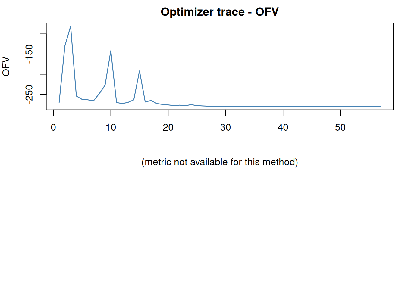
ferx_plot_trace() draws the OFV and each theta/omega/sigma parameter over iterations. A well-converged fit shows smooth descent with a stable plateau.
If you want the raw trace data:
tr <- ferx_trace(fit)
head(tr)
iter method phase ofv wall_ms grad_norm step_norm inner_iter_count
1 1 foce NA -269.86583 4 NA NA NA
2 2 foce NA -129.75853 5 NA 0.500000 NA
3 3 foce NA -81.30113 6 NA 0.707107 NA
4 4 foce NA -254.17371 10 NA 0.707107 NA
5 5 foce NA -262.46067 14 NA 0.707107 NA
6 6 foce NA -263.56191 18 NA 0.707107 NA
optimizer lm_lambda ofv_delta step_accepted cond_nll gamma mh_accept_rate
1 bobyqa NA NA NA NA NA NA
2 bobyqa NA NA NA NA NA NA
3 bobyqa NA NA NA NA NA NA
4 bobyqa NA NA NA NA NA NA
5 bobyqa NA NA NA NA NA NA
6 bobyqa NA NA NA NA NA NA
n_ebe_unconverged n_ebe_fallback
1 0 1
2 0 0
3 0 0
4 0 1
5 0 1
6 0 1ferx_trace() requires the fit to have been produced with optimizer_trace = TRUE (as in the fit at the top of this section); otherwise it errors with a clear message.
Run log and iteration history
ferx_runlog() prints a formatted run report that now includes a per-iteration history section (truncated for long runs). When you need the full, untruncated iteration table, ferx_runlog_iters() returns every iteration row without omission. Both require optimizer_trace = TRUE:
ferx_runlog(fit)        # formatted report; iteration history truncated for long runs
ferx_runlog_iters(fit)  # the complete, untruncated iteration table
Saving and reloading a fit
For long-running fits, persist the result to disk and reload later without re-fitting. The fit object embeds SHA-256 hashes of the model file and dataset so ferx_load_fit() warns you if either has changed since the fit was saved.
ferx_save_fit(fit, "warfarin.fitrx")           # data not embedded by default
ferx_save_fit(fit, "warfarin.fitrx", include_data = TRUE)

fit_reloaded <- ferx_load_fit("warfarin.fitrx")
include_data = TRUE embeds the dataset as a base64 blob so the .fitrx file is self-contained — useful for sharing a fit across machines.
Async fitting (ferx_fit_async / ferx_collect)
For long fits you can keep the R session free while the optimizer runs in the background:
handle <- ferx_fit_async(ex$model, ex$data, method = "saem", verbose = FALSE)
# ... do other work ...
fit <- ferx_collect(handle)   # block until done; shows live trace if verbose = TRUE
ferx_fit_async() returns a ferx_job handle immediately. ferx_collect(handle) blocks until the fit finishes and returns the same ferx_fit object you would get from ferx_fit(). In RStudio the job appears in the Jobs pane.
Note
ferx_fit_async() returns a job handle, not a fit object. Pass the handle to ferx_collect() to retrieve the completed fit:
fit <- ferx_collect(ferx_fit_async(...))Gradient method and $gradient_used
ferx_fit() accepts a gradient argument. The default uses the engine’s standard finite-difference gradient path.
The field fit$gradient_used tells you which gradient method the engine actually used: "fd" or "N/A" for methods that have no inner gradient (pure SAEM). Both print(fit) and summary(fit) display the requested and used methods side by side:
Gradient (requested): auto (used: fd)For a quick programmatic check:
fit$gradient_used          # "fd" | "N/A"
fit$gradient_method_inner  # raw engine label
fit$gradient_method_outer  # raw engine label for the outer loop
Common convergence issues
| Symptom | Likely cause | Fix |
|---|---|---|
| OFV oscillates | Step size too large | Lower maxiter; narrow bounds |
maxiter hit without convergence |
Model is misspecified | Check structural model; simplify |
| Covariance non-positive-definite | Over-parameterised | Remove insignificant ETAs or reduce model |
| Parameter hits bound | Bound too tight | Widen bounds; re-parameterise |
Comparing models
Use OFV differences for nested models (the likelihood ratio test) or AIC/BIC for non-nested:
fit_base <- ferx_fit(ex$model, ex$data)Mu-referencing detected for: ETA_CL, ETA_KA, ETA_V# A model with fixed ETA_KA (simpler)
ex_no_ka_bsv <- ferx_example("warfarin") # would use a modified model
# delta_ofv <- fit_base$ofv - fit_simpler$ofv
# p_value <- pchisq(delta_ofv, df = 1, lower.tail = FALSE)The chi-squared test with df = difference in number of parameters.