Quickstart
This chapter fits a one-compartment oral PK model to the bundled warfarin dataset. It covers the complete loop: data → model → fit → inspect → plot.
Load ferx
The example dataset
ferx_example() returns paths to a bundled model file and a NONMEM-format CSV. Calling it with no argument lists all bundled examples:
 [1] "bioavailability_ode"           "bioavailability"
 [3] "emax_pkpd"                     "igd_inverse_gaussian"
 [5] "mm_multistart"                 "mm_oral"
 [7] "one_cpt_iv_ode"                "one_cpt_iv"
 [9] "three_cpt_iv_ode"              "three_cpt_iv"
[11] "three_cpt_oral_ode"            "three_cpt_oral"
[13] "transit_2cpt"                  "two_cpt_iv_ode"
[15] "two_cpt_iv"                    "two_cpt_oral_cov_ode_template"
[17] "two_cpt_oral_cov_ode"          "two_cpt_oral_cov"
[19] "two_cpt_oral_derived"          "warfarin_additive_eta"
[21] "warfarin_addl"                 "warfarin_block_omega"
[23] "warfarin_bloq"                 "warfarin_data_selection"
[25] "warfarin_dcm"                  "warfarin_derived_pkpd"
[27] "warfarin_derived"              "warfarin_if"
[29] "warfarin_iov_saem"             "warfarin_iov"
[31] "warfarin_logit_f"              "warfarin_ltbs"
[33] "warfarin_ode_lagtime"          "warfarin_ode_time"
[35] "warfarin_ode"                  "warfarin_saem"
[37] "warfarin_scaled"               "warfarin_sde"
[39] "warfarin_ss"                   "warfarin"
ex <- ferx_example("warfarin")
ex$model
[1] "/home/runner/work/_temp/Library/ferx/examples/models/warfarin.ferx"
$data
[1] "/home/runner/work/_temp/Library/ferx/examples/data/warfarin.csv"Peek at the data:
  ID TIME      DV EVID AMT CMT RATE MDV
1  1  0.0       .    1 100   1    0   1
2  1  0.5  5.3653    0   .   1    0   0
3  1  1.0  8.2578    0   .   1    0   0
4  1  2.0 10.7063    0   .   1    0   0
5  1  4.0 11.4142    0   .   1    0   0
6  1  8.0 10.9232    0   .   1    0   0
The dataset follows the standard NONMEM column convention:
-
EVID = 1for dose records (with non-zeroAMT),EVID = 0for observations. -
MDV = 1masks a row from the likelihood (typically every dose row);MDV = 0for observed concentrations. -
CMTselects the compartment for dose / observation. For a one-compartment oral model with a single endpoint the dose lands in the absorption compartment and observations come from the central compartment — both areCMT = 1here because the analyticalone_cpt_oralsolver tracks them together. -
RATE = 0is a bolus dose; non-zeroRATEindicates an infusion (zero-order input).
DV values written as . (NONMEM convention for missing) are read by read.csv() as text; ferx parses them as NA internally.
The warfarin dataset bundled with ferx has 10 subjects and 110 observations after dose rows are excluded.
The model file
ferx_model_show(ex$model)# model: warfarin.ferx
# One-compartment oral PK model (warfarin)
[parameters]
theta TVCL(0.134, 0.001, 10.0)
theta TVV(8.1, 0.1, 500.0)
theta TVKA(1.0, 0.01, 50.0)
omega ETA_CL ~ 0.07
omega ETA_V ~ 0.02
omega ETA_KA ~ 0.40
sigma PROP_ERR ~ 0.01 (sd)
[individual_parameters]
CL = TVCL * exp(ETA_CL)
V = TVV * exp(ETA_V)
KA = TVKA * exp(ETA_KA)
[structural_model]
pk one_cpt_oral(cl=CL, v=V, ka=KA)
[error_model]
DV ~ proportional(PROP_ERR)
[fit_options]
method = foce
maxiter = 300
covariance = trueThe model DSL is described in detail in the Model file reference in the ferx-core book.
Fit the model
fit <- ferx_fit(model = ex$model, data = ex$data, verbose = FALSE)Mu-referencing detected for: ETA_CL, ETA_KA, ETA_Vverbose = FALSE silences per-iteration progress; omit it to watch the optimiser. Convergence is reached when the optimiser’s stopping criterion is met (gradient norm or function tolerance, depending on the optimiser).
Inspect results
summary(fit)--------------------------------------------------
ferx NLME Fit Summary
--------------------------------------------------
Model: warfarin
Dataset: warfarin
Converged: YES
Method: FOCEI
Gradient: auto (requested) -> analytic (Dual2) (used)
ferx v0.1.6 (core v0.1.6)
Settings (model file / call-time override):
method foce [model only]
maxiter 300 [model only]
covariance true [model only]
Structure: 1-cpt oral (TVCL, TVV, TVKA) | IIV: ETA_CL, ETA_V, ETA_KA | IOV: none | Residual: proportional
OFV: -285.9971 AIC: -271.9971 BIC: -253.0938
Subjects: 10 Obs: 110 Params: 7 Iter: 66
Shrinkage: ETA1=-0.4% ETA2=-0.1% ETA3=1.1%
EPS shrinkage: 14.9%
DW: 2.61 [negative autocorrelation]
lag-1 r: -0.365
Covariance: computed Cond: 1.0 | Wall time: 0.3s
Warnings:
* mu-ref: ETA_CL, ETA_KA, ETA_V
* Negative IWRES autocorrelation detected (Durbin-Watson = 2.61). Possible over-parameterization or misspecified error model.
* 24 EBE fallback(s)
--------------------------------------------------summary(fit) prints a compact run report: convergence, method, OFV/AIC/BIC, the auto-derived model structure (compartments, IIV, residual type), shrinkage, the Durbin-Watson autocorrelation statistic and lag-1 r, the gradient method requested and actually used, covariance status and condition number, wall time, and any active warnings. It also lists the [fit_options] actually in effect (model file vs. call-time overrides).
For the full parameter table including standard errors, use print(fit). The print(fit) layout leads with a prominent STATUS: CONVERGED line, followed by OFV/AIC/BIC, then bold-headed sections for THETA, OMEGA, SIGMA, SHRINKAGE, DIAGNOSTICS, and RUN INFO, and a warning-count footer that points you to ferx_warnings(fit) for remediation guidance:
print(fit)============================================================
NONLINEAR MIXED EFFECTS MODEL ESTIMATION
============================================================
Model: warfarin Dataset: warfarin
Method: FOCEI | Gradient: ANALYTIC (DUAL2) | Subjects: 10 | Obs: 110
STATUS: CONVERGED 66 iterations 0.3s
OFV: -285.9971 AIC: -271.9971 BIC: -253.0938
MODEL STRUCTURE (auto-derived)
------------------------------------------------------------
Structural: 1-cpt oral (TVCL, TVV, TVKA)
IIV: ETA_CL, ETA_V, ETA_KA
IOV: none
Residual: proportional
THETA
------------------------------------------------------------
Parameter Estimate SE %RSE
----------------------------------------------------
TVCL 0.132914 0.007081 5.3
TVV 7.727826 0.239060 3.1
TVKA 0.805940 0.149312 18.5
OMEGA (between-subject variability)
------------------------------------------------------------
ETA_CL [log-normal] = 0.028365 CV% = 17.0 SE = 0.012636
ETA_V [log-normal] = 0.009533 CV% = 9.8 SE = 0.004263
ETA_KA [log-normal] = 0.342926 CV% = 64.0 SE = 0.155138
SIGMA (residual error)
------------------------------------------------------------
PROP_ERR [proportional] = 0.010588 (var = 0.000112, CV% = 1.1) SE = 0.000839 [initial specified as SD]
SHRINKAGE
------------------------------------------------------------
ETA_CL: -0.4% ETA_V: -0.1% ETA_KA: 1.1% EPS: 14.9%
DIAGNOSTICS
------------------------------------------------------------
Covariance: computed Cond: 1.0 DW: 2.61 [negative autocorrelation] IWRES lag-1 r: -0.365
RUN INFO
------------------------------------------------------------
Gradient (requested): auto (used: analytic (Dual2))
ferx v0.1.6 (core v0.1.6)
SETTINGS (model file / call-time override)
------------------------------------------------------------
method foce [model only]
maxiter 300 [model only]
covariance true [model only]
------------------------------------------------------------
1 warning 1 info -- call ferx_warnings(fit) for details
============================================================For programmatic access, ferx_estimates() returns a tidy data frame:
ferx_estimates(fit) param transform estimate se rse_pct lower_95
1 TVCL identity 0.132914050 0.007081331 5.327752 0.119034641
2 TVV identity 7.727825893 0.239059541 3.093490 7.259269194
3 TVKA identity 0.805939683 0.149311939 18.526441 0.513288282
4 ETA_CL variance 0.028364800 0.012635963 44.548040 0.003598314
5 ETA_V variance 0.009533318 0.004263384 44.720885 0.001177085
6 ETA_KA variance 0.342926014 0.155138147 45.239539 0.038855246
7 PROP_ERR proportional 0.010587956 0.000838587 7.920196 0.008944326
upper_95 estimate_natural lower_95_natural upper_95_natural init_as_sd
1 0.14679346 NA NA NA FALSE
2 8.19638259 NA NA NA FALSE
3 1.09859108 NA NA NA FALSE
4 0.05313129 NA NA NA FALSE
5 0.01788955 NA NA NA FALSE
6 0.64699678 NA NA NA FALSE
7 0.01223159 NA NA NA TRUENotable columns:
-
transform— natural scale of the parameter (identity,variance,proportional, …). -
estimate,se,rse_pct— point estimate, standard error, and relative SE. -
lower_95,upper_95— asymptotic 95% confidence interval on the estimation scale. -
estimate_natural/lower_95_natural/upper_95_natural— back-transformed values where applicable (e.g. CV% from a log-normal omega). -
init_as_sd—TRUEif the model file declared the initial value on the SD scale ((sd)qualifier) rather than variance.
Individual diagnostics
Per-observation diagnostics live in fit$sdtab; per-subject EBEs in fit$ebe_etas.
head(fit$sdtab) ID TIME DV PRED IPRED CWRES IWRES EBE_OFV N_OBS
1 1 0.5 5.3653 4.272231 5.351960 0.4819160 0.23541634 -25.91287 11
2 1 1.0 8.2578 7.090919 8.283605 0.3974650 -0.29422145 -25.91287 11
3 1 2.0 10.7063 10.137289 10.708476 0.1496055 -0.01919035 -25.91287 11
4 1 4.0 11.4142 11.817021 11.383132 -0.5198810 0.25777812 -25.91287 11
5 1 8.0 10.9232 11.501752 10.757614 -0.5762295 1.45376895 -25.91287 11
6 1 12.0 9.9442 10.755788 10.069152 -0.8906758 -1.17202870 -25.91287 11
TAFD TAD
1 0.5 0.5
2 1.0 1.0
3 2.0 2.0
4 4.0 4.0
5 8.0 8.0
6 12.0 12.0head(fit$ebe_etas) ID ETA_CL ETA_V ETA_KA
1 1 0.028364174 0.06637554 0.3760943
2 2 0.015782650 -0.06287963 -0.4066030
3 3 -0.024295069 0.09140468 0.1583802
4 4 -0.028453158 -0.21097859 -0.7240953
5 5 -0.233831947 -0.12114034 0.4872084
6 6 -0.009959542 0.07080392 1.2524438Goodness-of-fit plots
The two most informative GOF plots are IPRED vs DV and CWRES vs PRED.
sdtab <- fit$sdtab

p1 <- ggplot(sdtab, aes(x = IPRED, y = DV)) +
  geom_point(alpha = 0.5) +
  geom_abline(slope = 1, intercept = 0, colour = "#1F6B7A") +
  labs(title = "IPRED vs DV", x = "Individual prediction", y = "Observed DV")

p2 <- ggplot(sdtab, aes(x = PRED, y = CWRES)) +
  geom_point(alpha = 0.5) +
  geom_hline(yintercept = 0, colour = "#1F6B7A") +
  geom_hline(yintercept = c(-2, 2), linetype = "dashed", colour = "#C8893E") +
  labs(title = "CWRES vs PRED", x = "Population prediction", y = "CWRES")

patchwork::wrap_plots(p1, p2)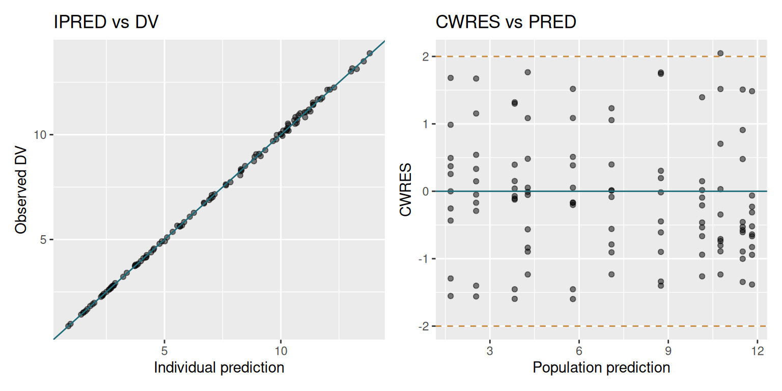
For a full treatment of diagnostics see Overview.
What’s next
-
Overview — pre-fit inspection and editing of
.ferxfiles -
Model file reference — understand every section of the
.ferxfile - Overview — fitting options, methods, and convergence
- Overview — full diagnostic suite and shrinkage
- Overview — simulate from the fitted model and overlay a VPC